
지난번 랜덤 포레스트 회귀 모델로 자전거의 일별 대여량을 예측하여 RMSE 점수 945가 나왔었다. 이번에는 하이퍼 파라미터 튜닝을 통하여 가능한 더 낮은 점수를 얻어볼 것이다.
4.1 데이터 셋 준비
1
2
3
from sklearn.model_selection import train_test_split
X_train, X_test, y_train, y_test = train_test_split(X_bikes, y_bikes,
                                                    random_state=2)
4.2 n_estimators
합리적인 n_estimators 값을 선택해보자. n_estimator를 증가시키면 시간과 비용이 늘어나지만 정확도는 향상시킬 수 있다.
1
2
3
4
5
6
7
8
9
10
11
12
13
14
15
16
17
18
19
20
21
22
23
24
25
26
27
from sklearn.metrics import mean_squared_error

rmse_scores = []
estimators = []

rf = RandomForestRegressor(warm_start=True, n_jobs=-1,
                           random_state=2)

est = 10

for i in range(21):
  rf.set_params(n_estimators=est)
  rf.fit(X_train, y_train)

  rmse = mean_squared_error(y_test, rf.predict(X_test), squared=False)

  rmse_scores.append(rmse)
  estimators.append(est)

  est += 25

plt.figure(figsize=(15, 7))
plt.plot(estimators, rmse_scores)
plt.xlabel('Number of Trees')
plt.ylabel('RMSE')
plt.title('Random Forest Bike Rentals', fontsize=15)
plt.show()
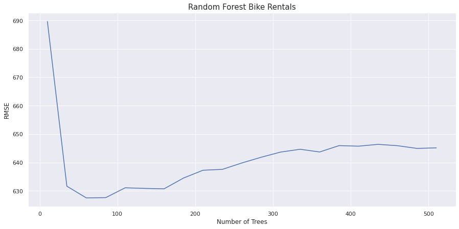
50개 언저리에서 가장 좋은 성능을 발휘한다. 100개가 넘어가면 에러가 상승하기 시작한다. 나중에 다시 살펴본다.
4.3 cross_val_score
위 그래프를 보면 RMSE 범위가 620에서 690사이이다. cross_val_score() 함수로 이 데이터셋에 대해 교차검증을 해보자. 교차 검증 함수는 훈련된 모델을 반환하지 않기 때문에 oob_score_를 확인 할 수 없다.
1
2
3
4
5
6
7
rf = RandomForestRegressor(n_estimators=50, warm_start=True,
                           n_jobs=-1, random_state=2)
scores = cross_val_score(rf, X_bikes, y_bikes,
                         scoring='neg_mean_squared_error', cv=10)
rmse = np.sqrt(-scores)
print(f'RMSE:{np.round(rmse, 3)}')
print(f'RMSE mean:{rmse.mean():.3f}')
RMSE:[ 836.482 541.898 533.086 812.782 894.877 881.117 794.103 828.968 772.517 2128.148] RMSE mean:902.398
이 점수는 이전보다 더 좋다. 그러나 RMSE 마지막 폴드의 에러가 매우 높다. 이는 데이터에 있는 오류나 이상치(outline) 때문일 수 있다.
4.4 하이퍼파라미터 튜닝
이제 RandomizedSearchCV로 하이퍼파라미터 튜닝을 수행해보자. 아래는 여러가지 하이퍼파라미터를 넣고 성능을 보기 위한 함수이다.
1
2
3
4
5
6
7
8
9
10
11
12
13
14
15
16
17
18
19
20
21
from sklearn.model_selection import RandomizedSearchCV
from sklearn.metrics import mean_squared_error as MSE

def randomized_search_reg(params, runs=16,
                          reg=RandomForestRegressor(random_state=2,n_jobs=-1)):
  rand_reg = RandomizedSearchCV(reg, params, n_iter=runs,
                                scoring='neg_mean_squared_error',
                                cv=10, n_jobs=-1, random_state=2)
  rand_reg.fit(X_train, y_train)

  best_model = rand_reg.best_estimator_
  best_params = rand_reg.best_params_
  print(f'best parameters: {best_params}')

  best_score = np.sqrt(-rand_reg.best_score_)
  print(f'train score: {best_score}')

  y_pred = best_model.predict(X_test)

  rmse_test = MSE(y_test, y_pred)**.5
  print(f'test score: {rmse_test:.3f}')
1트
초기 매개변수 그리드로 위 함수를 호출해 첫번쨰 결과를 확인한다
1
2
3
4
5
6
7
8
9
10
11
%%time
params = {
    'min_weight_fraction_leaf': [0, .0025, .005, .00785, .01, .05],
    'min_samples_split': [2, .01, .02, .03, .04, .06, .08, .1],
    'min_samples_leaf': [1, 2, 4, 6, 8, 10, 20, 30],
    'min_impurity_decrease': [0, .01, .05, .1, .15, .2],
    'max_leaf_nodes': [10, 15, 20, 25, 30, 35, 40, 45, 50, None],
    'max_features': ['auto', .8, .7, .6, .5, .4],
    'max_depth': [None, 2, 4, 6, 8, 10, 20]
}
randomized_search_reg(params)
best parameters: {‘min_weight_fraction_leaf’: 0, ‘min_samples_split’: 0.03, ‘min_samples_leaf’: 6, ‘min_impurity_decrease’: 0.05, ‘max_leaf_nodes’: 25, ‘max_features’: 0.7, ‘max_depth’: None} train score: 759.0756188493968 test score: 701.802 CPU times: user 1.1 s, sys: 68.4 ms, total: 1.17 s Wall time: 10 s
2트
탐색범위를 좁혀본다
1
2
3
4
5
6
7
8
%%time
params = {
    'min_samples_leaf': [1, 2, 4, 6, 8, 10, 20, 30],
    'min_impurity_decrease': [0, .01, .05, .1, .15, .2],
    'max_features': ['auto', .8, .7, .6, .5, .4],
    'max_depth': [None, 2, 4, 6, 8, 10, 20]
}
randomized_search_reg(params)
best parameters: {‘min_samples_leaf’: 1, ‘min_impurity_decrease’: 0.1, ‘max_features’: 0.6, ‘max_depth’: 10} train score: 679.0520498695299 test score: 626.541 CPU times: user 1.13 s, sys: 72.7 ms, total: 1.2 s Wall time: 10.2 s
3트
탐색횟수를 늘리고 max_depth를 더 늘려본다
1
2
3
4
5
6
7
8
%%time
params = {
    'min_samples_leaf': [1, 2, 4, 6, 8, 10, 20, 30],
    'min_impurity_decrease': [0, .01, .05, .1, .15, .2],
    'max_features': ['auto', .8, .7, .6, .5, .4],
    'max_depth': [None, 4, 6, 8, 10, 12, 15, 20]
}
randomized_search_reg(params, runs=20)
best parameters: {‘min_samples_leaf’: 1, ‘min_impurity_decrease’: 0.1, ‘max_features’: 0.6, ‘max_depth’: 12} train score: 675.1280049404816 test score: 619.014 CPU times: user 1.35 s, sys: 84.1 ms, total: 1.44 s Wall time: 12.9 s
4트:
이전 결과를 바탕으로 범위를 더 좁혀본다
1
2
3
4
5
6
7
8
%%time
params = {
    'min_samples_leaf': [1, 2, 3, 4, 5, 6],
    'min_impurity_decrease': [0, .01, .05, .08, .1, .12, .15],
    'max_features': ['auto', .8, .7, .6, .5, .4],
    'max_depth': [None, 8, 10, 12, 14, 16, 18, 20]
}
randomized_search_reg(params)
best parameters: {‘min_samples_leaf’: 1, ‘min_impurity_decrease’: 0.05, ‘max_features’: 0.7, ‘max_depth’: 18} train score: 679.5945071230298 test score: 630.954 CPU times: user 1.19 s, sys: 77.8 ms, total: 1.27 s Wall time: 10.9 s
에러가 늘어났으므로 여기서 멈추고, n_estimator나 더 늘려본다.
5트: 데이터 이상으로 인한 저조한 성능
n-estimators 늘려보기
1
2
3
4
5
6
7
8
9
%%time
params = {
    'min_samples_leaf': [1, 2, 4, 6, 8, 10, 20, 30],
    'min_impurity_decrease': [0, .01, .05, .1, .15, .2],
    'max_features': ['auto', .8, .7, .6, .5, .4],
    'max_depth': [None, 4, 6, 8, 10, 12, 15, 20],
    'n_estimators': [100]
}
randomized_search_reg(params, runs=20)
best parameters: {‘n_estimators’: 100, ‘min_samples_leaf’: 1, ‘min_impurity_decrease’: 0.1, ‘max_features’: 0.6, ‘max_depth’: 12} train score: 675.1280049404816 test score: 619.014 CPU times: user 1.34 s, sys: 113 ms, total: 1.45 s Wall time: 13.1 s
마지막으로 cross_val_score()로 결과를 확인해본다.
1
2
3
4
5
6
7
8
9
rf = RandomForestRegressor(n_estimators=100, min_impurity_decrease=.1,
                           max_features=.6, max_depth=12, n_jobs=-1,
                           random_state=2)

scores = cross_val_score(rf, X_bikes, y_bikes,
                         scoring='neg_mean_squared_error', cv=10)
rmse = np.sqrt(-scores)
print(f'RMSE:{np.round(rmse, 3)}')
print(f'RMSE mean:{rmse.mean():.3f}')
RMSE:[ 818.354 514.173 547.392 814.059 769.54 730.025 831.376 794.634 756.83 1595.237] RMSE mean:817.162
오잉?!?!? 점수가 더 나빠졌다.
cross_val_score()의 마지막 폴드의 점수가 다른 것보다 2배 가량 높기 때문에 마지막 폴드에 문제가 있다고 유추해볼 수 있다. 데이터를 다시 섞어서 시도해보자.
1
2
3
4
5
6
7
8
9
10
11
12
13
14
15
16
from sklearn.utils import shuffle

df_shuffle_bikes = shuffle(df_bikes, random_state=2)

X_shuffle_bikes = df_shuffle_bikes.iloc[:, :-1]
y_shuffle_bikes = df_shuffle_bikes.iloc[:, -1]

rf = RandomForestRegressor(n_estimators=100, min_impurity_decrease=.1,
                           max_features=.6, max_depth=12, n_jobs=-1,
                           random_state=2)

scores = cross_val_score(rf, X_shuffle_bikes, y_shuffle_bikes,
                         scoring='neg_mean_squared_error', cv=10)
rmse = np.sqrt(-scores)
print(f'RMSE:{np.round(rmse, 3)}')
print(f'RMSE mean:{rmse.mean():.3f}')
RMSE:[630.093 686.673 468.159 526.676 593.033 724.575 774.402 672.63 760.253 616.797] RMSE mean:645.329
기대한 대로 점수가 훨씬 좋아졌음을 알 수 있다.
4.5 랜덤 포레스트의 단점
결국 랜덤 포레스트는 개별 트리에 제약이 있다. 모든 트리가 동일한 실수를 저지르면 랜덤 포레스트도 실수를 한다. 앞의 사례에서 데이터를 섞기 전에 이런 경우가 있음을 보았다. 개별 트리가 해결할 수 없는 데이터 내의 문제 때문에 랜덤 포레스트의 성능이 향상될 수 없었다.
이럴 때 트리의 실수로부터 배워서 초반의 단점을 개선할 수 있는 앙상블 방법이 도움이 될 수 있다. 부스팅은 트리가 저지를 실수에서 배우도록 설계되었다.